Time sure flies.
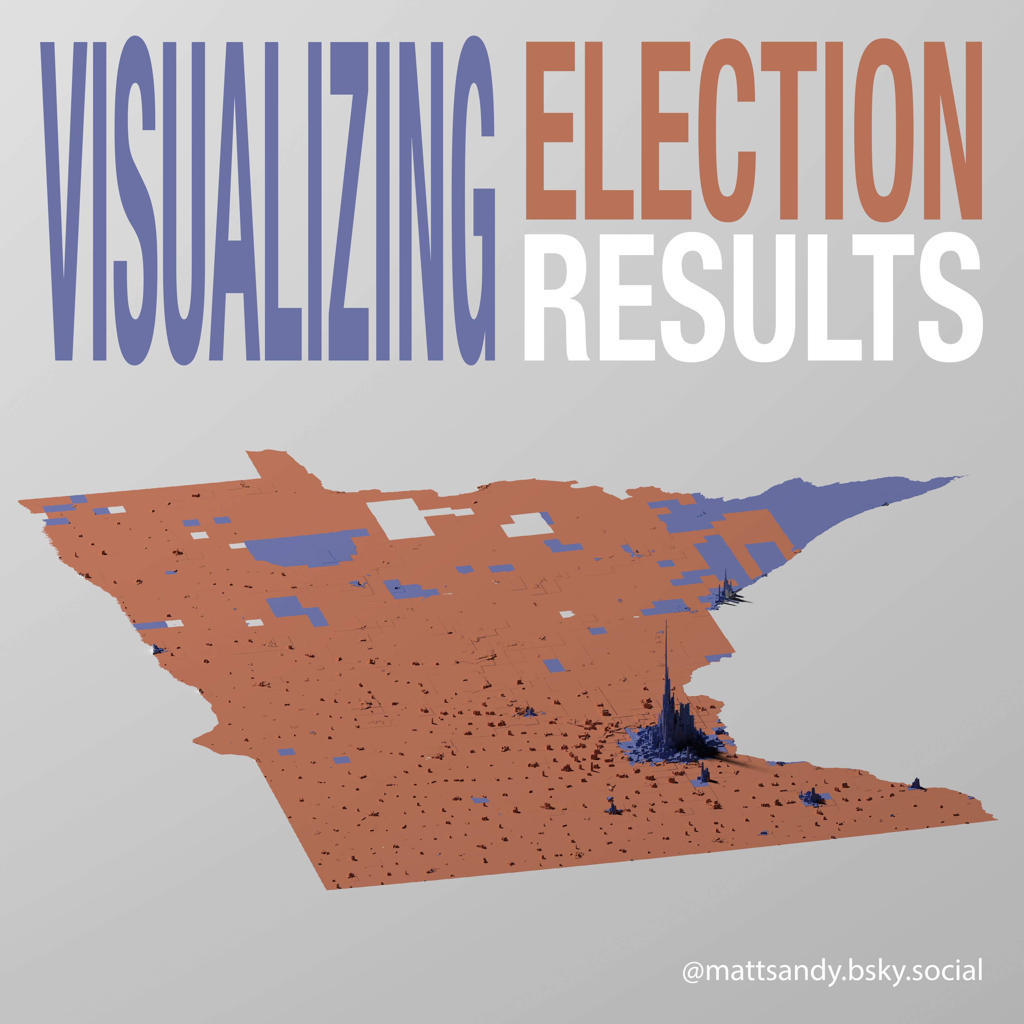
It has been a while since I have posted a tutorial, but I think I have a good one. The idea of 3d representations for population data has been around for some years, but I wanted to look exclusively at the winning votes after all other votes have been cancelled out.

Project Setup
We will need both the shapefile for the precinct as well as the election results for each precinct. Thankfully Minnesota provides a lot of transparency and the data is readily available. The shapefiles are available at gisdata.mn.gov, and the precinct level results are available at electionresults.sos.mn.gov.
Required Libraries
I typically will load more libraries than required, just because I like using them at some point.
1 2 3 4 5 6 7 8 | library(tidyverse) library(glue) library(jsonlite) library(sf) library(st) library(rayshader) library(rmapshaper) |
Geospatial Fun
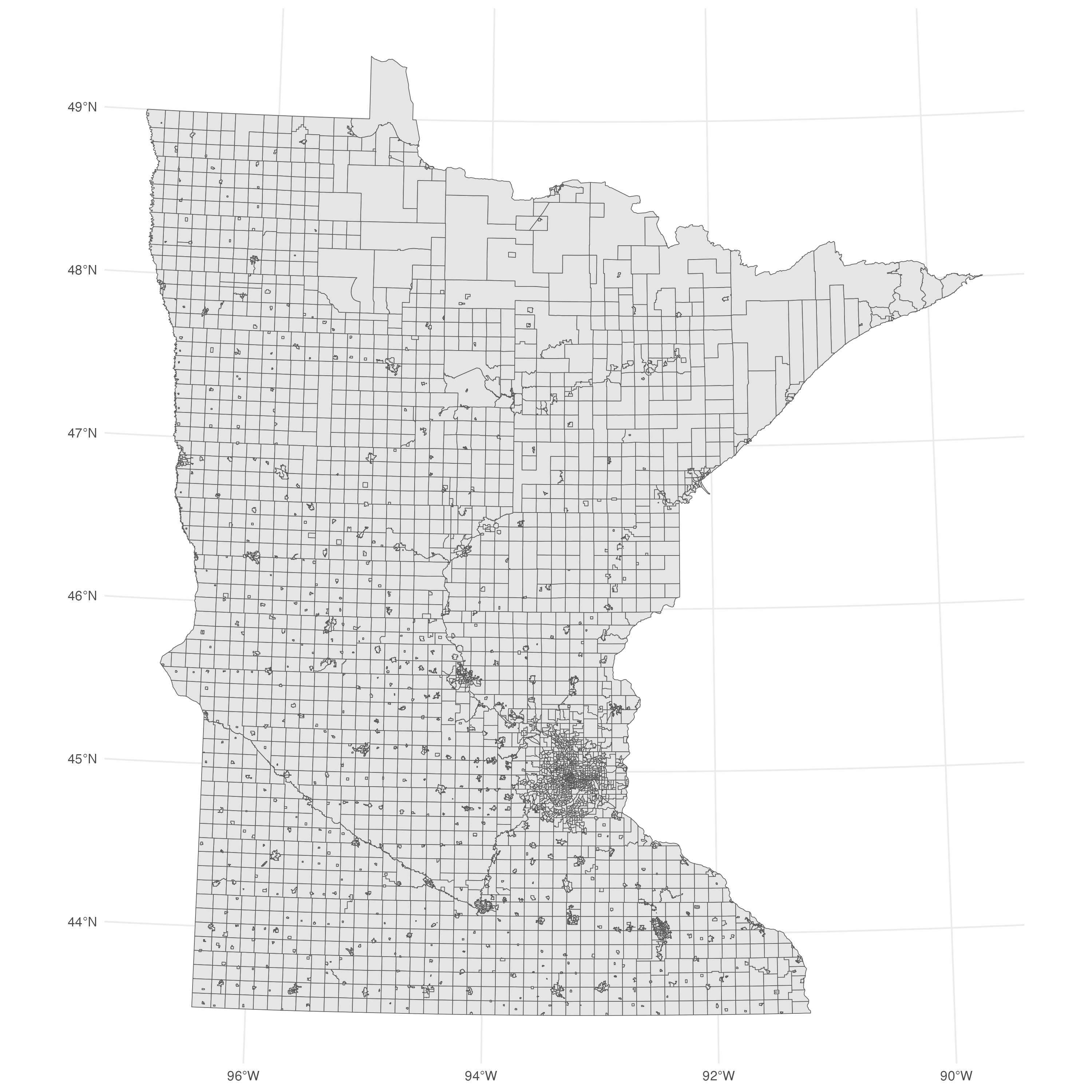
1 2 3 4 5 6 7 8 9 10 11 12 13 14 15 16 17 18 | # Read in shapefile voting_districts <- st_read("./shp_bdry_votingdistricts/bdry_votingdistricts.shp") |> janitor::clean_names() |> mutate( precinct_name = pctname |> toupper() |> str_remove_all("[^A-Z0-9]") ) |> mutate( precinct_id = pctcode, county_id = countycode |> as.numeric() ) # Plot with ggplot ggplot(voting_districts) + geom_sf() + theme_minimal() |
As you can see, the precinct_name has been capitalized while removing any non-alphanumeric characters. This is done to prevent potential issues when joining the election results.

Precinct Information
Now we need to read in the precinct data. I am reading directly from the url, but you can save the file locally to work offline. This data will be used to walk between the voting data and the geospatial data.
1 2 3 4 5 6 7 8 9 10 11 12 13 14 15 16 17 18 19 20 21 22 23 24 25 | precincts <- read_delim("https://electionresultsfiles.sos.mn.gov/20241105/PrctTbl.txt", delim = ";", col_names = FALSE) |> rename( county_id = X1, precinct_id = X2, precinct_name = X3, congressional_district = X4, legislative_district = X5, county_commissioner_district = X6, judicial_district = X7, soil_and_water_conservation_district = X8, mcd_fips_code = X9, school_district_number = X10 ) |> mutate( precinct_name = precinct_name |> toupper() |> str_remove_all("[^A-Z0-9]") ) |> select( county_id, precinct_id, precinct_name, mcd_fips_code ) |
As you can see, while after reading in the file I renamed all of the columns since the file didn’t contain a header. I pulled those columns from this description which contains the layout of many of the election result text files. As you can see, the precinct_name has been capitalized while removing any non-alphanumeric characters. This is done to prevent potential issues when joining the geospatial results.
Voting Information
Once again, thank goodness for that media layout file above that describes the columns. As you can see, the voting file contains precinct_id and county_id. There was no need to read in the precinct file. Sometimes that happens, and time is spent down a rabbit hole you never needed to go down. That is okay though.
1 2 3 4 5 6 7 8 9 10 11 12 13 14 15 16 17 18 19 20 21 22 23 24 25 26 27 28 29 30 31 32 33 34 35 36 37 38 39 40 41 42 43 44 45 46 47 48 49 50 | votes <- read_delim("https://electionresultsfiles.sos.mn.gov/20241105/USPresPct.txt", delim = ";", col_names = FALSE) |> rename( state = X1, county_id = X2, precinct_id = X3, office_id = X4, office_name = X5, district = X6, candidate_order_code = X7, candidate = X8, suffix = X9, incumbent_code = X10, party_abbreviation = X11, precincts_reporting = X12, total_precincts = X13, vote_count = X14, vote_percentage = X15, total_votes = X16 ) |> # We are only looking at two candidates filter( candidate %in% c( "Donald J. Trump and JD Vance", "Kamala D. Harris and Tim Walz" ) ) |> group_by( county_id, precinct_id ) |> select( county_id, precinct_id, vote_count, candidate ) |> # Renaming the candidate values mutate( candidate = case_when( candidate == "Kamala D. Harris and Tim Walz" ~ "Harris", 1 == 1 ~ "Trump" ), county_id = county_id |> as.numeric() ) |> pivot_wider( names_from = candidate, values_from = vote_count, values_fn = sum # Add this line to sum up duplicate vote counts ) |
Building the initial Matrix
You can make this larger, which will look better. I am keeping this at 2000 for simplicity’s sake. This mat will be used a couple more times, once for the color/fill and once for the elevation matrix.
1 2 3 4 5 6 7 8 9 10 11 12 13 14 15 16 17 18 19 20 21 22 23 24 25 26 27 28 | # Calculate bounding box dimensions bbox <- st_bbox(joined) # Get bounding box w_ratio <- (bbox$xmax - bbox$xmin) / (bbox$ymax - bbox$ymin) h_ratio <- 1 # Height ratio (adjust if needed) size <- 2000 # Define the desired raster size # Define raster dimensions nx <- floor(size * w_ratio) # Number of columns ny <- floor(size * h_ratio) # Number of rows # Rasterize Population Data with st_rasterize dmv_rast <- stars::st_rasterize( joined["winning_vote_land_area"], # Specify the column to rasterize dx = (bbox$xmax - bbox$xmin) / nx, # Cell width dy = (bbox$ymax - bbox$ymin) / ny # Cell height ) dim(dmv_rast) dmv_rast$winning_vote_land_area |> max(na.rm = TRUE) # ------------------------------------------------------------------------- # Convert to matrix for use in visualization mat <- as.matrix(dmv_rast[["winning_vote_land_area"]]) mat[is.na(mat)] <- 0 # Replace NA values with 0 dim(mat) |
Building Additional Matrices
We will need both a color matrix and an elevation matrix.
Color Matrix
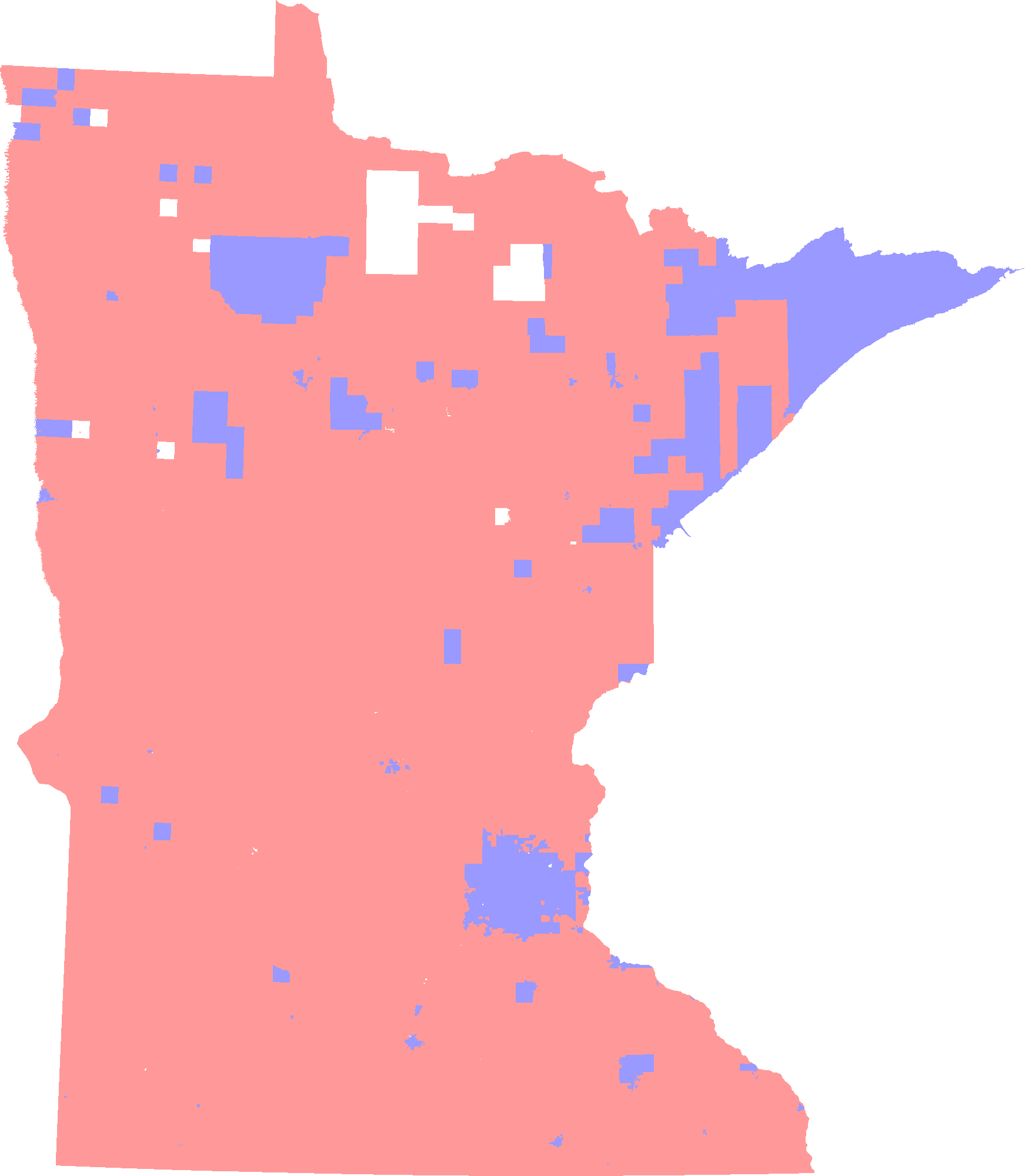
1 2 3 4 5 6 7 8 9 10 11 12 13 14 15 16 17 18 19 20 21 22 23 24 25 26 27 28 29 30 31 32 | # Dimensions of the matrix nrow_mat <- nrow(mat) ncol_mat <- ncol(mat) # Initialize a 4D RGBA matrix (Rows x Columns x RGBA channels) # Added 4th dimension for alpha rgba_matrix <- array(NA, dim = c(nrow_mat, ncol_mat, 4)) # Assign RGB and Alpha values # Three possible outcomes (red, blue, or white) for (i in 1:nrow_mat) { for (j in 1:ncol_mat) { if (is.na(mat[i, j]) || mat[i, j] == 0) { # White: RGB = (1, 1, 1), Alpha = 0.9 rgba_matrix[i, j, ] <- c(1, 1, 1, 1) } else if (mat[i, j] > 0) { # Blue: RGB = (0, 0, 1), Alpha = 0.9 rgba_matrix[i, j, ] <- c(0, 0, 1, 0.4) } else { # Red: RGB = (1, 0, 0), Alpha = 0.9 rgba_matrix[i, j, ] <- c(1, 0, 0, 0.4) } } } # Flip and rotate matrix rgba_matrix <- aperm(rgba_matrix, c(2, 1, 3)) dim(rgba_matrix) # Save rbaa matrix as png # This is a sanity check png::writePNG(rgba_matrix, "dmv_raster.png") |
The export should show a rasterized version, and the white fills are where Trump and Harris tied in total votes for those precincts.

Elevation Matrix
Now for the elevation matrix
1 2 | elevation_matrix <- abs(mat) |
Yeah, that was easy. Winning votes are winning votes, whoever they are for. Elevation, in the context of this plot, should always be positive.
Positioning, Rendering, and Saving
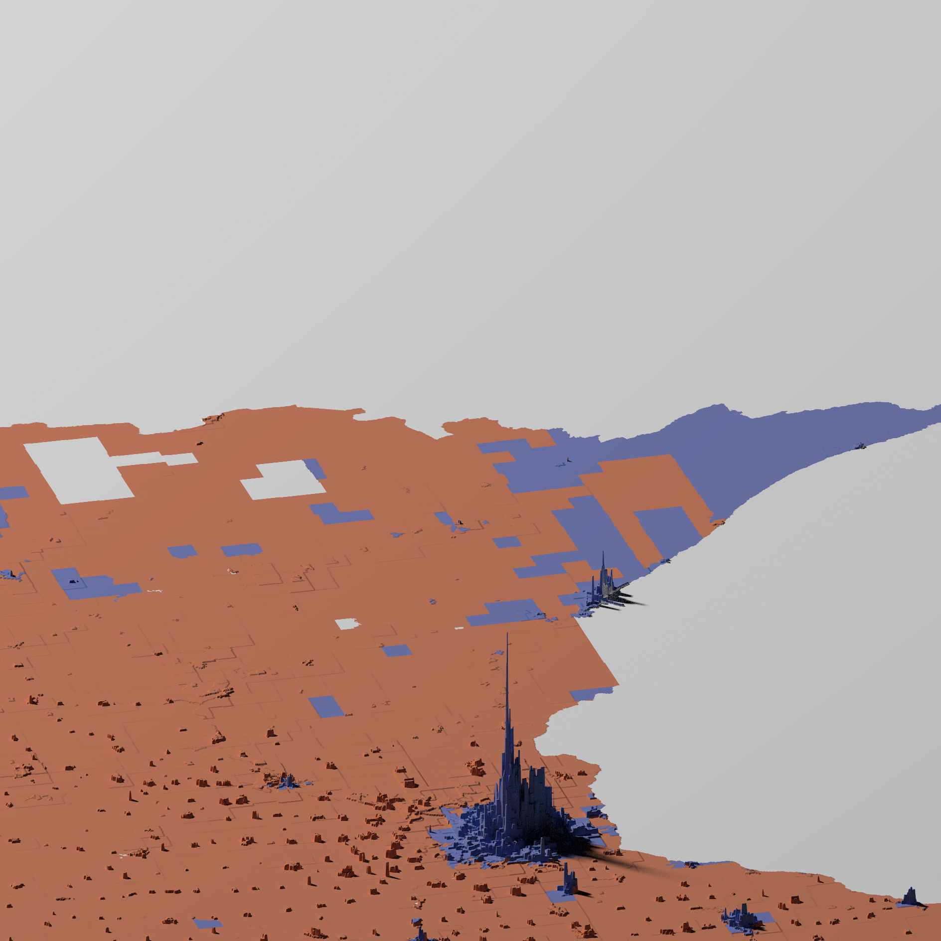
1 2 3 4 5 6 7 8 9 10 11 12 13 14 15 16 17 18 19 20 21 22 23 24 25 | # Plot the matrix elevation_matrix |> #height_shade(texture = texture) |> sphere_shade() |> add_overlay(overlay = rgba_matrix) |> plot_3d( heightmap = elevation_matrix, zscale = 20, solid = FALSE, shadowdepth = 0 ) # Render Camera render_camera(theta = -15, phi = 24, zoom = .7) # Save High-Quality Render render_highquality( filename = "plot.png", width = 1920*2, height = 1920*2, interactive = FALSE, light = TRUE ) |
This is only a fraction of the power of https://www.rayrender.net/. Be sure to check that site out and the render_highquality reference. This tutorial was inspired by https://justjensen.co/making-population-density-maps-with-rayrender-in-r/.


Be First to Comment