
This tutorial will mainly focus on ggplot and bigrams, but it does gloss over clustering for a heatmap.
This project started a while back, tweeting the plots at the beginning of this month. Life happens I suppose. Bought a new bike, had a birthday, yaddayadda. Better late then never?
I want to preface this with the disclaimer that a phrase repeated isn’t inherently good or bad. Emphasis through repetition is sometimes needed to drive a point home.
Required Libraries
First step, as always, is to include the libraries we will be using.
1 2 3 4 5 6 7 8 9 10 11 12 13 14 15 16 | # Always Included library(tidyverse) library(magrittr) # Plotting library(ggplot2) library(ggthemes) # String manipulation library(stringr) # Tokenization library(quanteda) # Heatmap rescaling require(scales) library(dplyr) # Just for melt() library(data.table) |
Define Candidates
This appends the candidates from the second debate to the candidates of the first debate.
1 2 3 4 5 6 7 8 9 10 11 12 13 14 15 16 17 18 19 20 | candidates <- c("Sanders", "Klobuchar", "Warren", "Buttigieg", "O'Rourke", "Bullock", "Delaney", "Ryan", "Williamson") %>% append(c("Bennet", "Gillibrand", "Castro", "Booker", "Harris", "Biden", "Yang", "Gabbard", "Inslee", "de Blasio")) %>% toupper |
Reading the Transcripts
I ended up grabbing the transcripts from nbcnews.com and saving as a CSV file after some regex cleaning. I couldn’t find both days on their site anymore, so I am linking to the CNN transcripts
I also kept the transcripts separate just in case I needed to refer to Night One and Night Two separately down the road. Once I read them in I noticed some white space and that I still needed to remove the ‘:’ character.
1 2 3 4 5 6 7 8 9 10 | transcriptA <- read_csv("2019-07-30.csv",col_names = F,trim_ws = T,quote = '"') names(transcriptA) <- c("person","dialog") transcriptA$person %<>% str_replace_all(":","") transcriptA$dialog %<>% trimws transcriptB <- read_csv("2019-07-31.csv",col_names = F,trim_ws = T,quote = '"') names(transcriptB) <- c("person","dialog") transcriptB$person %<>% str_replace_all(":","") transcriptB$dialog %<>% trimws |
Now that we have Transcript A and B ready in and using the same column names, we can bind them.
1 2 | transcript <- rbind(transcriptA,transcriptB) |
If we wanted to keep our workspace clean, this would be an excellent opportunity to save the transcripts in a list (transcript$A and transcript$B). Using that method would allow you to use transcript$Full <- transcript %>% bind_rows which looks cleaner.
Working with Bigrams
This part might get a little overwhelming, but essentially this chunk of code will
- Loop through each individual candidate
- Subset the transcript by current candidate
- Loop through Dialog of current subset
- Return bigrams
- Generate frequency table of returned bigrams
- Add column for current candidate
The reason we are nesting an lapply instead of collapsing is to prevent the end of a sentence to be used with the beginning of a new sentence (ex: “He fell in. The boy cried” shouldn’t include the bigram “IN_THE”). While generating n-grams on each dialog separately won’t prevent this, it will reduce occurrences.
If you want to further improve upon this code, you could split the dialog by punctuation marks c('?', '!', '.', ';').
1 2 3 4 5 6 7 8 9 10 11 12 13 14 15 16 | bigrams <- lapply(unique(transcript$person),function(candidate) { lapply(transcript %>% filter(person==candidate) %>% .[["dialog"]], function(text) { text %>% str_remove_all('\\.\\.\\.') %>% tokens(remove_numbers = TRUE, remove_punct = TRUE) %>% tokens_select(pattern = stopwords('en'), selection = 'remove') %>% tokens_ngrams(n = 2) %>% toupper %>% unique }) %>% unlist %>% table %>% data.frame -> df if(nrow(df)>0) { df$Candidate <- candidate return(df) } else { return(NULL) } }) names(bigrams) <- unique(transcript$person) |
If you want to give the results a test, you can use
1 2 | bigrams$WARREN %>% top_n(n = 10, wt = Freq) |
1 2 3 4 5 6 7 8 9 10 11 12 13 14 | . Freq Candidate 1 ACROSS_COUNTRY 3 WARREN 2 AROUND_WORLD 5 WARREN 3 CARE_SYSTEM 3 WARREN 4 COURAGE_FIGHT 3 WARREN 5 DONALD_TRUMP 8 WARREN 6 ENTIRE_WORLD 3 WARREN 7 FIGHT_BACK 4 WARREN 8 GOD-GIVEN_RIGHT 3 WARREN 9 HEALTH_CARE 7 WARREN 10 INSURANCE_COMPANIES 3 WARREN 11 RIGHT_NOW 6 WARREN 12 UNITED_STATES 5 WARREN |
Pretty cool, right?
Bigrams, Extended
Now that we have everything all nice and segmented, we will be merging everything into one big table bigram_table to plot.
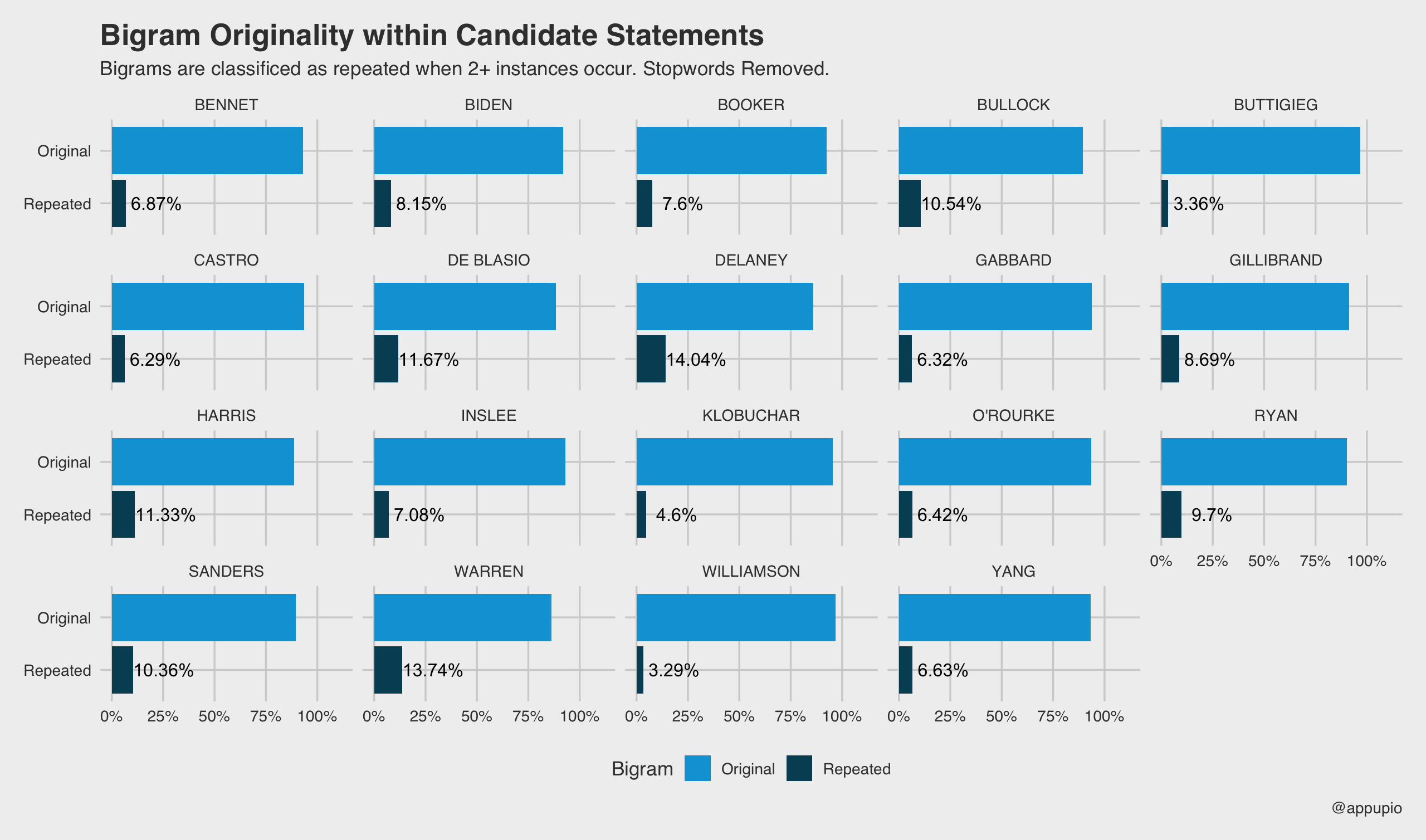
1 2 3 4 5 6 7 8 9 10 11 12 13 14 15 | bigram_table <- bigrams %>% bind_rows # Renaming, but only the first column is changed names(bigram_table) <- c("Gram","Freq","Candidate") # Filter out non-candidates (announcer) bigram_table %<>% filter(Candidate %in% candidates) # Create new column bigram_table$Repeat <- ifelse(bigram_table$Freq>1,"Repeated","Original") # Now some grouping to determine percentages bigram_table <- bigram_table %>% group_by(Candidate,Repeat) %>% summarise(n = sum(Freq)) %>% mutate(Percentage = (n / sum(n))*100) # Label column added, but only will show repeated bigram_table$Label <- NA bigram_table$Label[bigram_table$Repeat=="Repeated"] <- bigram_table$Percentage[bigram_table$Repeat=="Repeated"] %>% round(digits = 2) %>% paste0("%") |
Plotting Originality
1 2 3 4 5 6 7 8 9 10 11 12 13 14 15 16 17 18 19 20 21 22 23 24 | ggplot(bigram_table, aes(x = factor(Repeat,levels=c("Repeated", "Original")), y = Percentage, label = Label, fill = Repeat)) + geom_bar(stat="identity") + coord_flip() + scale_y_continuous(breaks = c(0,25,50,75,100), labels = c("0%", "25%", "50%", "75%", "100%")) + geom_text(nudge_y = 15) + theme_fivethirtyeight() + scale_fill_economist() + facet_wrap(~Candidate) + labs(title = "Bigram Originality within Candidate Statements", subtitle = paste0("Bigrams are classificed as repeated when ", "2+ instances occur. ", "Stopwords Removed."), caption = "@appupio", fill = "Bigram") |
Cool!
Heatmap
Clustering Bigrams
This next part is going to be a lot of piping, and I am sure someone has a much better way of doing things.
First we going to overwrite bigrams table with a fresh bind_rows call on the bigrams list.
1 2 3 4 5 | bigram_table <- bigrams %>% bind_rows %>% select(Gram = '.', Freq, Candidate) %>% filter(Candidate %in% candidates) |
I did the part above a little different than the first time. There are a handful of ways to rename columns of a data frame. Using select is a very nice alternative.
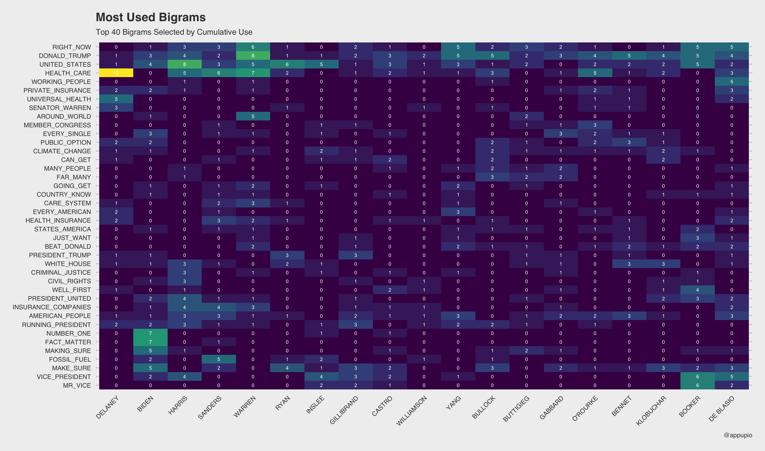
For the next part we will want to figure out what bigrams to use. I am selecting the top 40 used the most cumulatively among all candidates. We only need a vector of the actual grams.
1 2 3 4 5 6 | top_grams <- bigram_table %>% group_by(Gram) %>% summarise(Freq = sum(Freq)) %>% .[rev(order(.$Freq)),"Gram"] %>% unlist %>% as.vector |
To give that a test we can use
1 2 | top_grams[1:10] |
Looks like what we are looking for; let’s move on.
1 2 3 4 5 6 | [1] "DONALD_TRUMP" "UNITED_STATES" [3] "HEALTH_CARE" "RIGHT_NOW" [5] "MAKE_SURE" "AMERICAN_PEOPLE" [7] "VICE_PRESIDENT" "RUNNING_PRESIDENT" [9] "WHITE_HOUSE" "INSURANCE_COMPANIES" |
Time to filter bigram_table and convert to a matrix.
1 2 3 4 5 6 7 8 9 10 11 12 13 14 15 16 17 18 | cluster_matrix <- bigram_table %>% filter(Gram %in% top_grams[1:40]) %>% group_by(Gram,Candidate,Freq) %>% spread(Candidate,Freq) cluster_matrix[is.na(cluster_matrix)] <- 0 # numerical columns dat <- cluster_matrix[,2:(ncol(cluster_matrix))] %>% as.data.frame row.names(dat) <- cluster_matrix$Gram # clustering row.order <- hclust(dist(dat))$order col.order <- hclust(dist(t(dat)))$order # re-order matrix accoring to clustering dat_new <- dat[row.order, col.order] # reshape into dataframe cluster_matrix <- melt(as.matrix(dat_new)) names(cluster_matrix) <- c("Gram", "Candidate","Freq") |
Uff-da. Now that all of that is over, we can plot cluster_matrix.
Plotting the Heatmap
Lots of ways to style the heatmap, but I am going with a viridis heatmap and including those frequency within the cells. Sometimes you also want numbers.
1 2 3 4 5 6 7 8 9 10 11 12 13 14 15 | ggplot(cluster_matrix,aes(x = Candidate, y = Gram, fill = Freq, label = Freq)) + geom_tile() + scale_fill_viridis_c() + geom_text(color="#FFFFFF",size=2) + theme_fivethirtyeight() + theme(axis.text.x = element_text(angle = 45, hjust = 1)) + theme(legend.position="none", text = element_text(size=9)) + labs(title = "Most Used Bigrams", subtitle = "Top 40 Bigrams Selected by Cumulative Use", caption = "@appupio") |
Be First to Comment